PHYS250: Machine Learning

By Rahul Jakati & Alexander Miroshnichenko

Introduction

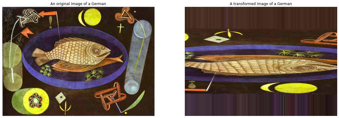
“Wow, what a fine piece of impressionism!” You glance nervously at your watch, wondering how your friend convinced you to come to the art gallery. You have no idea how to tell the difference between a piece of surrealism and romanticism, much less post-impressionism! Enter the machine learning project Alex and I have been working on for the past week. We adapted a pre-trained neural network(s) to distuinguish paintings by nationality and genre.

As a general overview of this post

1. Approach: A generalized summary of the concepts and data analysis which made up the model itself
2. Results: An analysis of the results generated from our two neural networks
3. Acknowledgements: People we would like to thank, as well as a link to the sources we have used

Approach

Here we detail our approach towards the construction of our model, including the actual frameworks and datasets used, as well as some of the conceptual understanding behind them.

Libraries

In our model we used the following datasets:

• Keras

• Tensorflow

• Pandas

• NumPy

• Seaborn

• Keras and Tensorflow are intertwined, two very popular libraries that contain the framework for the layers which made up our neural network.

• Pandas is a data manipulation library we used to assign labels to the images within our dataset

• Numpy is a mathematical library used to convert our images into tensors compatible as inputs into our model

• Seaborn is a graphing library similar to matplotlib, but with added visual effects and functions, which we used to generate the connfusion matrix

Data Processing

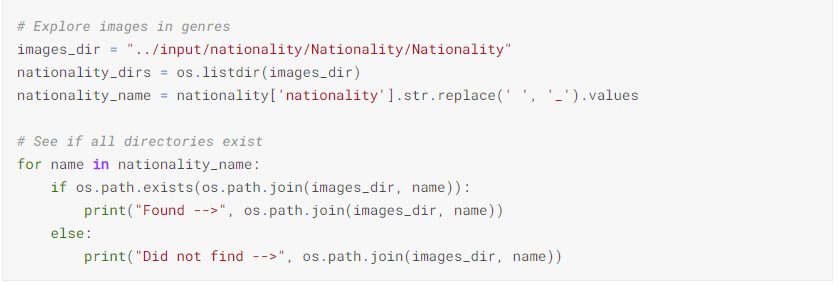
To assign labels to each image, the dataset had to be sorted.

We sorted the image dataset by hand into their respective nationalities and genres to assign labels to each image.

Using the os.listdir command, we were able to check each label and make sure that they were assigned correctly.

A fundamental problem of many datasets is normalization, especially when some labels within a dataset are present at a much higher frequency than others. We accounted for this using class weights. A nationality which includes many paintings will have lower class weights assigned to each painting, and vice versa for say, genres with a low amount of paintings.

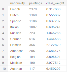
Image Augmentation

After processing the data, we wanted to introduce more pictures for the model to interpret, but without the hassle of scraping websites for painting data. We instead visually augmented the pictures we already had in various ways, including zooming in on a specific portion, mirroring, and even rotating the image. This massively increases the diversity of our dataset, and thus helps to prevent overfitting.

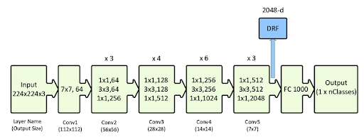
Resnet50

The model used for this project was a pre-trained neural network called Res-Net 50, which had been previously trained over 14 million images from the dataset Imagenet.. This allows for the weights to be more easily transferred to paintings due to the concept of transfer learning. It also results in massively reduced computational times, as the model can pick up patterns much quicker than a fresh model, due to having encountered those features before as part of its Imagenet training.

Model Parameters

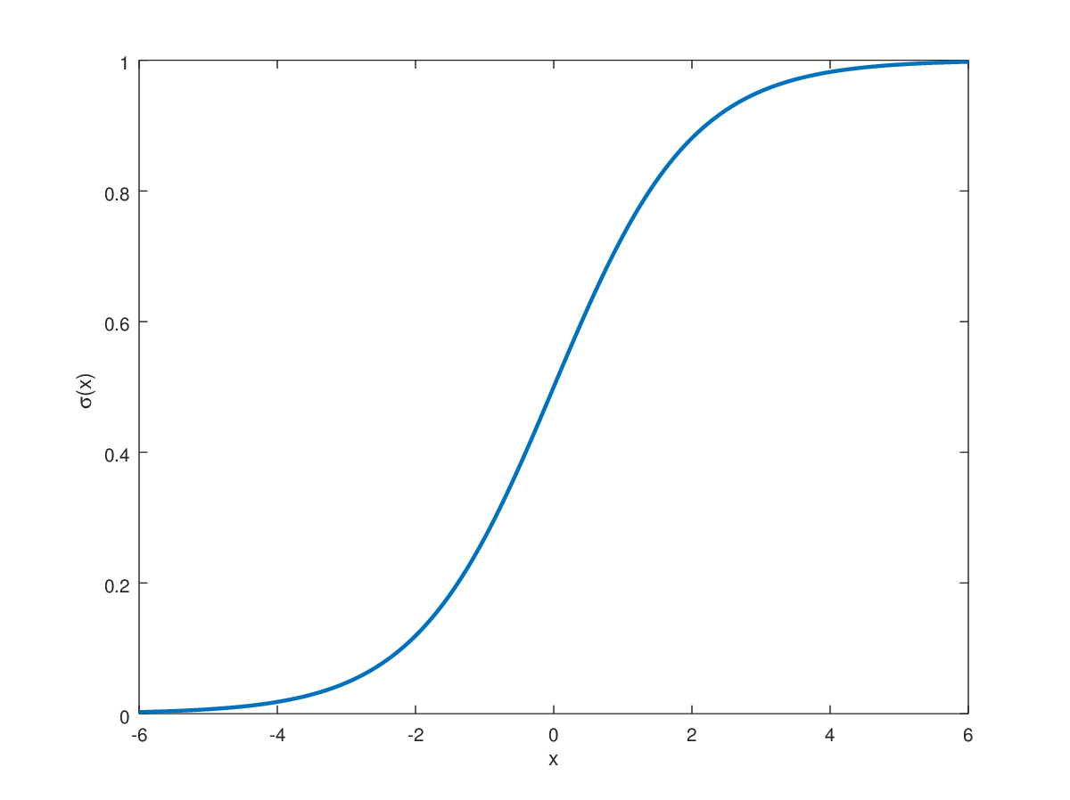
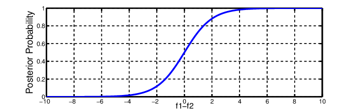
In a neural network, the outputs are typically a list of numbers that must be converted to percentages using an activation function. There are two main activation functions in deep learning, Softmax and Sigmoid, both of which are representations of logistic regression. In fact, if you look at the image below, I doubt you would be able to tell the difference (The top image is sigmoid). The difference lies in that Softmax is generalized to multiple dimensions, which usually makes it ideal for taking multiple inputs and spitting out a single output. However, we found that changing our activation function to sigmoid significantly increased validation accuracy as well decreasing loss by a significant amount. This may be due to the fact that probabilities of a label within each node do not necessarily have to add up to one when using the sigmoid equation, meaning that each label is independent of each other.

Another choice was our loss function. Due to the multi-class nature of the project, there are realistically only two possible options: Categorical Cross Entropy and Binary Cross Entropy. Binary Cross Entropy is typically used when there are more than one labels associated with each class, which was not the case in this project, despite our best efforts. In the future, we do want to run our model again, with categorical cross entropy instead.

Results

After training the models we adapted, we reflected on how well our model worked.

Accuracy and Loss

Accuracy is a measure of how many correct guesses the computer has in percent. If a computer has a 100% accuracy, then it is guessing 100% of the images correctly. Loss on the other hand is an optimization function which shows how well the model is fitting the data. The lower the loss, the better the model is fitting our data and the more accurate it should be.

Our image dataset was split into several different chunks, the training set and the validation set, we will have two different accuracies and losses for each network we made. The training set would be fed to the computer so that it could teach itself to find the differences between genres and nationalities. Afterwards, the computer would test itself on the validation set to confirm whether it was being correctly trained. This process would repeat, in our case, for about 35 epochs. As the network saw the training images while trying to learn off of them, the training accuracy should be higher than the validation accuracy and the training loss lower than the validation loss.

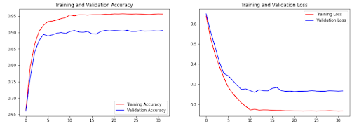
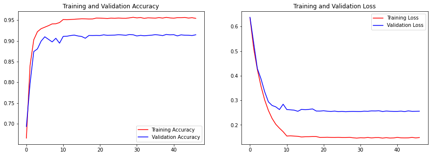
It is easily discernible that the training accuracy improved to around 95% and validation accuracy to 90% for both models. The losses also decreased significantly for both sets.

This is good… right? Well, maybe not so much.

One thing to note about our dataset is that the image accuracy began at around 70% correct for both models. This means that even off of the first training set, the network was able to correctly distinguish genres and nationalities much much better than by random chance, which is what we expected the first epoch to have an accuracy of. This could be a product of training a pretrained model, but it could also mean overfitting.

Overfitting is when a network finds details in an image set that don’t necessarily relate to what it’s looking for. For example, if a computer is training to distinguish between different animals and only sees images of sheep on green hills, it may think that the green hill is what defines a sheep and not the white fluffy animal on the hill. In essence, the network becomes too good at identifying the images in its training and validation sets to be able to correctly identify other images it comes across. Thus, our network may have found something other than what we call genre and nationality to differentiate between the two.

Confusion Matrices

A confusion matrix shows how “confused” the computer gets between different labels. The bottom of the matrix shows the labels that the computer guessed and the left side shows the actual labels. The number in each square of the matrix where the two labels (the guess and the actual answer) intersect is the recall percentage of those labels.

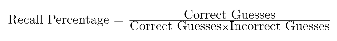
One thing to take note of is that the recall percentages in a row do not have to add up to 100%.

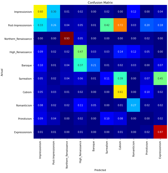
For our genre classification, the network did the best on the northern renaissance style of art. We are not quite sure why northern renaissance is the most easily selected from the dataset. Another very intriguing thing is that cubism was often confused for post-impressionism. Although cubism is an extension of post-impressionism, humans tend to see the geometric nature of cubism as very distinct and unique out of all of the genres. It is very odd that the network did not pick up on the shape of cubism but was able to aptly identify the intricacies of northern renaissance art. However, there is one genre in which the computer significantly underperformed: primitivism. This is most likely due to that primitivism is very similar to several other genres including impressionism, post-impressionism, expressionism, surrealism and high renaissance. It is almost a mixture of all of those genres and thus very difficult to distinguish on its own.

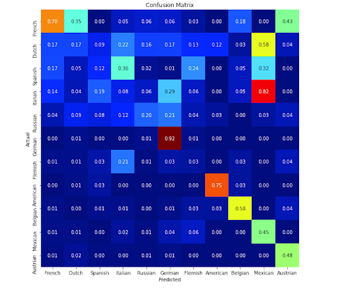
For our nationality classification, the network most easily identified German paintings. This could be because most of the German images we had in our dataset were very distinct and this allowed the computer to pick up on the unique nature of how these Germans painted. The very intriguing part of this matrix is that the network confused Mexican art for Italian and Dutch art. We are not really sure as to why the computer decided that Mexican art was close to these two nationalities, but we think it may have to do with the fact that many of the Italian renaissance paintings and some Dutch paintings were murals and a fair amount of the Mexican paintings were also murals.

Overall, these classification matrices seem to confirm one thing, that our network was in fact not able to correctly guess paintings 90% of the time and that something fishy was going on in the training of our network. In fact, for the nationality matrix, you can see that there are 5 nationalities which have a recall percentage that doesn’t reach above 20%. However, the best way to see whether our network worked was to test it on images.

Example Classifications

We took some images from the training and validation sets that the network had previously seen to first test the network. This would give us a baseline to see whether the computer had actually learned something or was not as good as we thought it was.

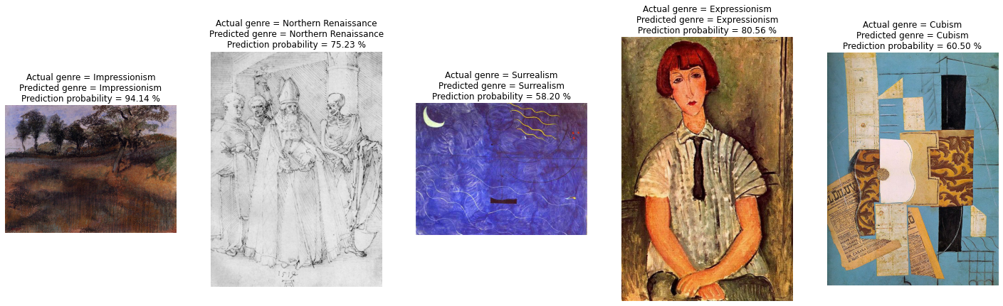
You can easily see how the computer was very confident in all of its answers and got all of the genres correct. This is either an indicator of a well trained network or an overfitted network.

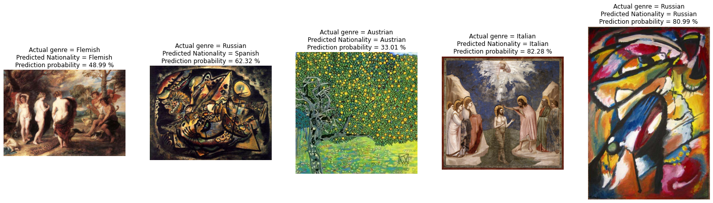
The computer was not as sure in these answers as it was in genres. The computer incorrectly guessed on genre probably because this Russian painting was not in the style of most other Russian paintings.

Only after testing it on images that it has not seen before will we be able to know whether the network correctly learned to differentiate between genres.

Test Paintings

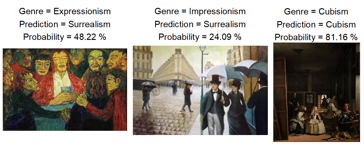
Now we took paintings outside of our dataset to test the network.

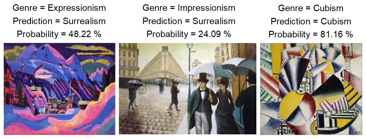
The network did not perform nearly as well as it had on the example classifications. Here, the computer incorrectly identified two of the three paintings. The first expressionist painting was in between surrealism and expressionism so it makes sense why the computer didn’t classify it correctly. The second painting, the computer was very unsure as to the style so it ended up also in surrealism. However, the third painting was a very distinct style of cubism which the computer confidently identified.

We can easily see that the computer is very confident in selecting German paintings. However, it also correctly identified the French painting of Paris. It misidentified the Spanish painting as Russian, but at least it got the majority of our test paintings correct.

Looking Forward

Looking forward, we have several objectives we want to improve this project on.

• Creating one multi-label classification network We plan to combine the two networks we have made into one. We want to assign two labels per image. We plan to do this by having all of the labels in one row and telling the computer that it has to pick the highest percentage out of the first half (genres) and the highest percentage out of the second half (nationalities).

• Introducing more genres/nationalities This will increase the versatility of the dataset. With more categories like Abstract Impressionism and Australian paintings, this network could prove to be more useful in more situations.

• Getting a bigger dataset to reduce the problems with overfitting Having more data is not guaranteed to solve our problem with overfitting, but it may help to relax the issue. Having a roughly equal amount of paintings in each genre/nationality will allow the computer to weigh all of them equally and not look into certain images more. This should reduce the issues we had with overfitting.

Acknowledgements

We would first like to thank Supratim Haldar, whose Kaggle Notebook called DeepArtist was invaluable in helping us make our model, and helped teach us how many of the concepts behind many of the libraries he used with his helpful commentary on his notebook. We would also like to thank the website LearnDataScience, whose article on multi-label classification was invaluable in teaching us how it worked and the principles behind it. Finally, we’d like to thank Donald Smith, for guiding us along the process the entire way.

A list of the sources we used: Sources